AutoML Guide

Endgame provides a full AutoML system that automatically profiles data, checks quality, selects and trains models, tunes hyperparameters, builds ensembles, optimizes thresholds, generates explanations, and produces a structured performance report — all behind a single fit / predict call.

Import convention: import endgame as eg

---

Architecture

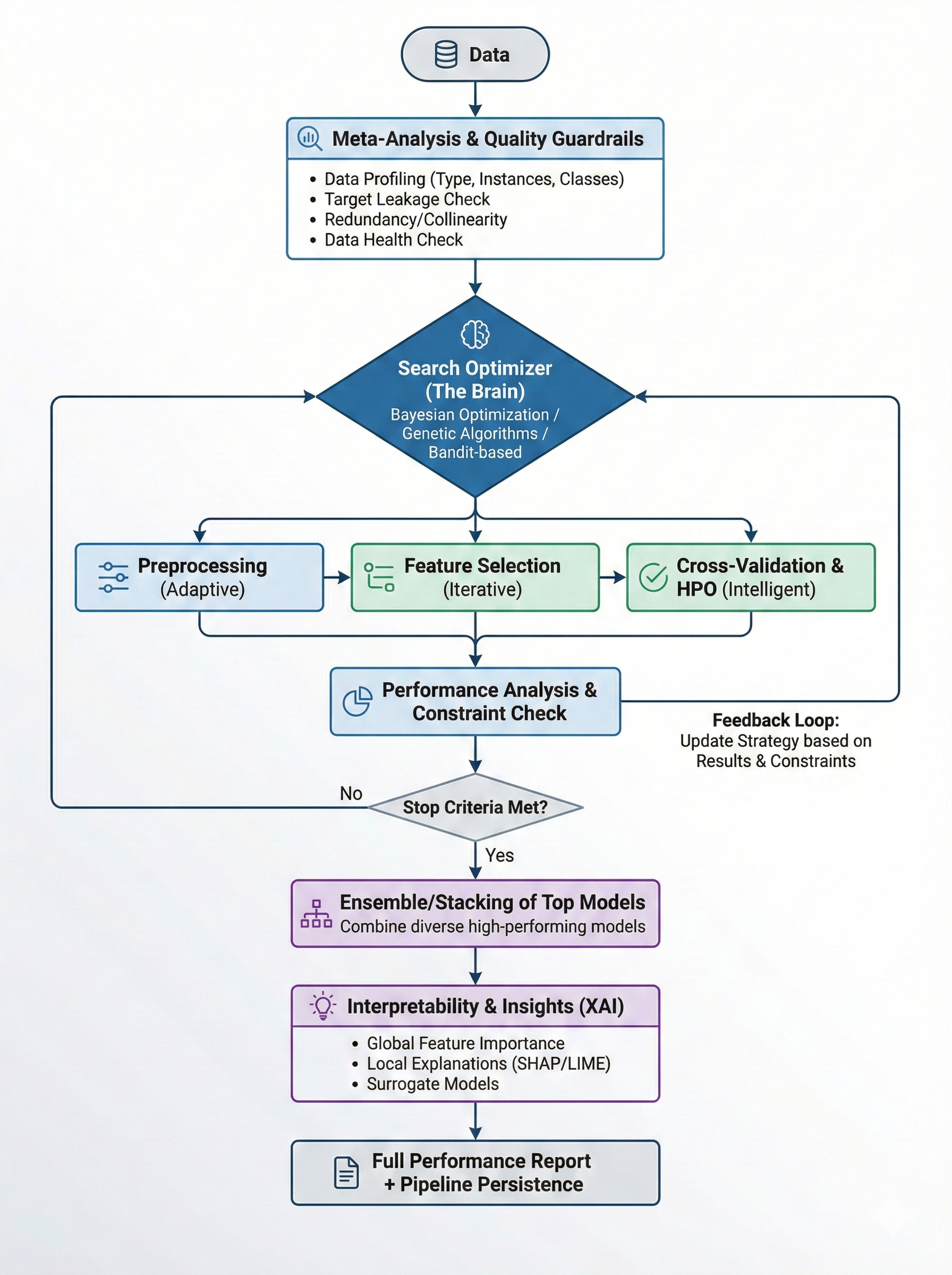
The AutoML pipeline executes 16 stages with intelligent time budget management. Each stage receives a fraction of the total time budget and unused time is automatically redistributed to later stages.

#	Stage	Purpose
1	Profiling	Extract dataset meta-features (size, types, class balance, correlations)
2	Quality Guardrails	Detect target leakage, feature redundancy, data health issues
3	Data Cleaning	Handle missing values, remove constant columns
4	Preprocessing	Encoding, scaling, imputation
5	Feature Engineering	Aggregations, interactions, polynomial features
6	Data Augmentation	SMOTE, ADASYN for imbalanced datasets
7	Model Selection	Search strategy suggests model configurations
8	Model Training	Train models with cross-validation from 76 registered models
9	Constraint Check	Validate models against deployment constraints (latency, size)
10	Hyperparameter Tuning	Optuna-based HPO for top-3 models
11	Ensembling	Hill climbing, stacking, blending, rank averaging, or auto-selection
12	Threshold Optimization	Optimize classification decision thresholds on OOF predictions
13	Calibration	Probability calibration (Platt, isotonic, temperature scaling)
14	Post-Training	Knowledge distillation, conformal prediction
15	Explainability	SHAP feature importances and feature interactions
16	Persistence	Save trained models and pipeline artifacts to disk

After the linear pipeline completes, a feedback loop can run up to 3 additional iterations if time permits — updating the search strategy with results, suggesting new model configurations, and re-running ensembling with all models.

When keep_training=True, the pipeline enters a continuous optimization loop that alternates between model search, training, optional HPO, and re-ensembling until convergence or interruption.

A performance report is generated after the pipeline finishes, summarizing the full run with leaderboard, stage timing, quality warnings, tuning results, and top features.

---

Quick Start

from endgame.automl import TabularPredictor

predictor = TabularPredictor(label="target", presets="best_quality")
predictor.fit(train_df)

y_pred  = predictor.predict(test_df)
y_proba = predictor.predict_proba(test_df)

predictor.leaderboard()

leaderboard() returns a pandas.DataFrame ranked by validation score, one row per trained model:

                 model  val_score  fit_time_s  pred_time_s
0        LGBMWrapper      0.9312       14.2         0.04
1         XGBWrapper      0.9287       18.6         0.06
2       FTTransformer      0.9241       92.0         0.31
3   HillClimbingEnsemble  0.9341        2.1         0.41

---

Constructor Parameters

TabularPredictor accepts the following parameters:

Parameter	Type	Default	Description
label	str	(required)	Name of the target column
problem_type	str	"auto"	"auto", "binary", "multiclass", or "regression"
eval_metric	str	"auto"	Evaluation metric ("roc_auc", "accuracy", "rmse", "mae", "log_loss", "f1", "r2", or a callable)
presets	str	"medium_quality"	Quality preset (see Preset System)
time_limit	int | None	None	Time budget in seconds. None uses preset default
search_strategy	str	"portfolio"	Search strategy (see Search Strategies)
track_experiments	bool	True	Track experiments to the meta-learning database
output_path	str | None	None	Path to save outputs (models, logs)
random_state	int	42	Random seed for reproducibility
verbosity	int	2	Verbosity level (0=silent, 1=progress, 2=detailed, 3=debug)
logger	ExperimentLogger | None	None	Experiment logger instance (e.g. MLflow)
constraints	DeploymentConstraints | None	None	Deployment constraints (latency, model size)
guardrails_strict	bool	False	Abort on critical quality issues instead of warning
checkpoint_dir	str | None	None	Directory for incremental checkpoints. Saves top-N models after key stages
keep_training	bool	False	Enable continuous optimization loop after main pipeline
patience	int	5	Consecutive rounds without improvement before stopping (continuous loop). Set to 0 for unlimited
min_improvement	float	1e-4	Minimum score improvement to count as progress
min_model_time	float	300.0	Minimum time budget (seconds) per model. Stops training stage if remaining time is less than this
max_model_time	float	600.0	Hard ceiling (seconds) per model. Prevents slow models from monopolizing the budget
excluded_models	list[str] | None	None	Model names to exclude from the search
early_stopping_rounds	int	50	Early stopping patience for GBDT models (LightGBM, XGBoost, CatBoost) during CV
use_gpu	bool	False	Enable GPU acceleration for supported models

predictor = TabularPredictor(
    label="target",
    presets="best_quality",
    time_limit=7200,
    checkpoint_dir="checkpoints/",
    keep_training=True,
    patience=10,
    min_improvement=1e-5,
    excluded_models=["saint", "tabpfn"],
    early_stopping_rounds=100,
)
predictor.fit(train_df)

---

Preset System

The preset argument controls the quality / speed trade-off. Seven built-in presets are available:

Preset	Description	Default time	CV folds	Ensemble	HPO
'best_quality'	Maximum accuracy, all model families	No limit	8	Auto (6 methods)	100 trials
'high_quality'	High accuracy, most model families	4 hours	5	Auto (6 methods)	50 trials
'good_quality'	Balanced speed and quality	1 hour	5	Auto (6 methods)	25 trials
'medium_quality'	Fast with reasonable quality (default)	15 min	5	Auto (6 methods)	10 trials
'fast'	GBDTs only, no HPO or ensembling	5 min	3	None	None
'interpretable'	Glass-box models only (EBM, GAM, rules, trees)	15 min	3	None	25 trials
'exhaustive'	Evolutionary search over all models + preprocessing + ensembles	No limit	3	Auto (6 methods)	Genetic

# Fast experiment — good for initial data exploration
predictor = TabularPredictor(label="target", presets="fast")
predictor.fit(train_df)

# Competition-grade — leave running overnight
predictor = TabularPredictor(label="target", presets="best_quality")
predictor.fit(train_df)

# Regulatory/compliance — interpretable models only
predictor = TabularPredictor(label="target", presets="interpretable")
predictor.fit(train_df)

Each preset defines time allocations for all 16 pipeline stages, curated model pools, and search budgets. See endgame/automl/presets.py for full details.

---

Prediction Methods

TabularPredictor provides four prediction methods:

predict(data, model=None)

Returns point predictions. For classification, applies threshold optimization automatically when available (trained during the threshold optimization stage on OOF predictions). For regression, returns raw predicted values.

y_pred = predictor.predict(test_df)

# Use a specific model instead of the ensemble
y_pred = predictor.predict(test_df, model="lgbm_standard")

predict_proba(data, model=None)

Returns probability predictions for classification tasks. Applies calibration automatically when a calibrator was fitted during the calibration stage.

y_proba = predictor.predict_proba(test_df)  # shape (n_samples, n_classes)

predict_sets(data, alpha=0.1)

Returns conformal prediction sets (classification) or prediction intervals (regression) with statistical coverage guarantees. Requires a preset that enables conformal prediction (best_quality or high_quality with validation data).

# 90% coverage prediction sets
pred_sets = predictor.predict_sets(test_df, alpha=0.1)

# Classification: boolean array (n_samples, n_classes) — True = class in set
# Regression: array (n_samples, 2) — [lower_bound, upper_bound]

predict_distilled(data)

Returns predictions from the lightweight distilled student model, trained via knowledge distillation from the ensemble teacher. Faster inference while approximating ensemble accuracy.

y_fast = predictor.predict_distilled(test_df)

---

Search Strategies

Eight search strategies are available:

Strategy	Description
'portfolio'	Diverse model portfolio with heuristic ranking (default)
'heuristic'	Data-driven rules based on meta-features
'genetic'	Evolutionary optimization of full pipelines (model + preprocessing + hyperparameters)
'random'	Random valid pipeline sampling
'bayesian'	Optuna-based Bayesian optimization
'bandit'	Successive Halving multi-fidelity search
'adaptive'	Meta-strategy: Portfolio → Bayesian on stagnation

predictor = TabularPredictor(
    label="target",
    presets="good_quality",
    search_strategy="bayesian",
)
predictor.fit(train_df)

Bandit Search (Successive Halving)

The 'bandit' strategy implements multi-fidelity optimization via Successive Halving. Many configurations are trained cheaply on small data fractions, and only the top performers are promoted to progressively larger fractions. This is far more time-efficient than training every configuration on the full dataset.

• Rung 0: Train all configurations on ~11% of data

• Rung 1: Promote top 1/3 to ~33% of data

• Rung 2: Promote top 1/3 to 100% of data

The reduction factor (eta=3) controls how aggressively configurations are pruned at each rung.

predictor = TabularPredictor(
    label="target",
    presets="good_quality",
    search_strategy="bandit",
)
predictor.fit(train_df, time_limit=1800)

Adaptive Search

The 'adaptive' strategy is a meta-strategy that switches between sub-strategies based on performance feedback:

1. Phase 1 — Portfolio: Diverse model sweep for broad coverage (first 15 rounds)

2. Phase 2 — Bayesian: Focused HPO on top performers (unlimited rounds)

The switch happens early when the current strategy stagnates (no improvement for 5 consecutive rounds).

predictor = TabularPredictor(
    label="target",
    presets="high_quality",
    search_strategy="adaptive",
)
predictor.fit(train_df, time_limit=3600)

Genetic / Evolutionary Search

The 'genetic' strategy treats the entire pipeline as a genome and evolves it using tournament selection, crossover, and mutation. Each individual encodes:

• Model choice and hyperparameters

• Preprocessing steps (imputation strategy, scaling, encoding)

• Feature selection method and top-k count

• Dimensionality reduction (PCA, none)

predictor = TabularPredictor(
    label="target",
    presets="good_quality",
    search_strategy="genetic",
)
predictor.fit(train_df, time_limit=3600)

The genetic search is most effective with longer time budgets (30+ minutes) where it has room for multiple generations. For quick experiments, 'portfolio' or 'heuristic' converge faster.

---

Quality Guardrails

The guardrails stage runs early in the pipeline and checks for:

• Target leakage — features with |correlation| > 0.95 with the target

• Feature redundancy — feature pairs with |correlation| > 0.98

• Data health — constant columns, all-missing columns, too few samples, extreme feature-to-sample ratio, minority class < 1%, ID-like columns

By default, issues are logged as warnings and the pipeline continues. To abort on critical issues:

predictor = TabularPredictor(
    label="target",
    presets="good_quality",
    guardrails_strict=True,  # Abort on critical issues
)
predictor.fit(train_df)

Quality warnings are included in the performance report:

report = predictor.report()
for warning in report.quality_warnings:
    print(f"[{warning.severity}] {warning.message}")

---

Deployment Constraints

Specify deployment constraints to automatically filter out non-compliant models:

from endgame.automl import TabularPredictor, DeploymentConstraints

predictor = TabularPredictor(
    label="target",
    presets="good_quality",
    constraints=DeploymentConstraints(
        max_predict_latency_ms=10.0,   # Max 10ms per 100-sample batch
        max_model_size_mb=50.0,        # Max 50MB serialized
        require_interpretable=False,   # Allow black-box models
    ),
)
predictor.fit(train_df)

The constraint check stage runs after model training and before HPO, measuring prediction latency and model size for each trained model. Non-compliant models are flagged in the report but still available for inspection.

---

Intelligent CV Selection

The pipeline automatically selects the most appropriate cross-validation strategy based on data characteristics:

Data Characteristic	CV Strategy	Notes
Time series detected	PurgedTimeSeriesSplit	Uses purging and embargo to prevent lookahead
Group column present	StratifiedGroupKFold	Keeps groups intact across folds
Small dataset (< 500 samples)	RepeatedStratifiedKFold / RepeatedKFold	3 repeats for stable estimates
Imbalanced classification	StratifiedKFold	Preserves class balance in each fold
Default classification	StratifiedKFold	Standard stratified k-fold
Default regression	KFold	Standard k-fold

The strategy is chosen once per run and applied consistently across all model evaluations. The number of folds is set by the preset (e.g. 8 for best_quality, 5 for good_quality, 3 for fast).

---

Hyperparameter Tuning

When enabled in the preset (hyperparameter_tune=True), the HPO stage selects the top-3 models by CV score and tunes them with Optuna. Tuning spaces are defined per model in the model registry (e.g., lgbm_standard, xgb_standard, catboost_standard).

The time budget for HPO is divided evenly across the top models. If tuning improves a model’s score, the tuned version replaces the original.

# HPO is enabled by default for good_quality and above
predictor = TabularPredictor(label="target", presets="good_quality")
predictor.fit(train_df, time_limit=3600)

# Check tuning results
report = predictor.report()
for entry in report.tuning_summary:
    print(f"{entry['model']}: {entry['original_score']:.4f} → {entry['tuned_score']:.4f}")

---

Ensembling

After individual models are trained, TabularPredictor builds an ensemble. When the preset uses ensemble_method="auto" (default for most presets), all six ensemble methods are tried and the best is selected by OOF score:

Method	Description
Hill climbing	Forward model selection optimizing the evaluation metric
Stacking	Meta-learner trained on out-of-fold predictions
Optimized blend	Optuna-optimized blending weights
Power blend	Score-proportional power weighting
Rank averaging	Rank-based blending for heterogeneous predictions
Uniform averaging	Simple equal-weight averaging (baseline)

The fast and interpretable presets disable ensembling (ensemble_method="none") to prioritize speed and interpretability respectively.

Ensembling runs after HPO and threshold optimization, so it operates on the best available versions of each model.

---

Threshold Optimization

For classification tasks, the threshold optimization stage finds optimal decision thresholds using out-of-fold predictions. This is particularly valuable for imbalanced datasets where the default 0.5 threshold is suboptimal.

The optimized thresholds are automatically applied in predict() when available. This is transparent — no code changes needed.

---

Continuous Training

When keep_training=True, the predictor enters a continuous optimization loop after the main pipeline completes. This loop alternates between:

1. Model search — ask the search strategy for new configurations

2. Training — fit the suggested configurations with CV

3. Optional HPO — run Optuna on the best models if time permits

4. Re-ensembling — rebuild the ensemble with the expanded model pool

The loop runs until one of:

• patience consecutive rounds without improvement exceeding min_improvement

• Total time_limit reached

• KeyboardInterrupt (saves checkpoint and exits gracefully)

# Run until convergence with periodic checkpoints
predictor = TabularPredictor(
    label="target",
    presets="exhaustive",
    keep_training=True,
    patience=10,
    min_improvement=1e-5,
    checkpoint_dir="checkpoints/",
)
predictor.fit(train_df)

Set patience=0 for truly unlimited optimization (useful with search_strategy="genetic" or "exhaustive" preset).

---

Early Stopping for GBDTs

Gradient-boosted decision tree models (LightGBM, XGBoost, CatBoost) use early stopping during cross-validation to avoid training unnecessary boosting rounds. A validation set from each CV fold monitors performance, and training halts when no improvement is seen for early_stopping_rounds consecutive rounds.

This is enabled by default (early_stopping_rounds=50) and applies only during CV scoring — the final refit on all data trains for the full n_estimators.

# Increase patience for noisy datasets
predictor = TabularPredictor(
    label="target",
    presets="best_quality",
    early_stopping_rounds=100,
)
predictor.fit(train_df)

---

GPU Support

Set use_gpu=True to enable GPU acceleration for models that support it (e.g. XGBoost, LightGBM, CatBoost, PyTorch-based neural models).

predictor = TabularPredictor(
    label="target",
    presets="best_quality",
    use_gpu=True,
)
predictor.fit(train_df)

When GPU mode is enabled:

• CUDA is validated at startup; a warning is emitted if no GPU is detected

• Training uses thread-based execution instead of fork to avoid CUDA re-initialization issues

• If a model encounters a CUDA out-of-memory error, it automatically falls back to CPU for that model

• When use_gpu=False (default), CUDA_VISIBLE_DEVICES="" is set to force CPU-only mode in worker processes

---

Model Interpretability

After fitting, inspect the learned structures of trained models:

display_models()

Prints rules, trees, equations, scorecards, coefficients, and feature importances for every trained model.

predictor = TabularPredictor(label="target", presets="interpretable")
predictor.fit(train_df)

# Display all trained models
text = predictor.display_models()

display_model(name)

Display the learned structure of a single model:

# Display a specific model's rules/structure
predictor.display_model("ebm")
predictor.display_model("rulefit")

Both methods accept top_rules (max rules/terms per model, default 15) and top_features (max features per importance display, default 10).

---

Explainability

The explainability stage computes SHAP-based feature importances for the best model using a subsample of the training data. Results are stored in the predictor and the performance report.

predictor.fit(train_df)

# Access explanations
explanations = predictor.explain()
print("Top features:", explanations["top_features"])
print(explanations["feature_importance_df"])

---

Performance Report

After fitting, a structured AutoMLReport is generated automatically. It contains:

• Summary — preset, time limit, total time, best score, number of models

• Stage summary — per-stage timing and success status

• Model leaderboard — all trained models ranked by score

• Quality warnings — issues detected by the guardrails stage

• Feature importances — SHAP-based importances from the explainability stage

• Tuning summary — per-model HPO results (original vs tuned score)

• Constraint violations — deployment constraint failures

predictor.fit(train_df)

# Get the report object
report = predictor.report()

# Print as markdown
print(report.to_markdown())

# Or convert to dict for programmatic access
data = report.to_dict()

# Display to stdout
report.display()

HTML Reports

Generate self-contained HTML reports with embedded CSS — no external dependencies required:

report = predictor.report()

# Get HTML string
html = report.to_html(title="My Experiment")

# Save directly to file
report.save_html("report.html", title="My Experiment")

The HTML report includes the full leaderboard, stage timing breakdown, quality warnings, feature importances chart, and tuning results in a styled, printable format.

---

Feedback Loop

When the preset enables HPO and time remains after the linear pipeline, a feedback loop runs up to 3 additional iterations:

1. Update the search strategy with all results collected so far

2. Suggest 2 new model configurations not yet tried

3. Train them with 50% of remaining time

4. Merge results and re-run ensembling

This iterative refinement is automatic and requires no configuration. It activates when at least 60 seconds remain in the time budget.

---

Task Inference

TabularPredictor infers the task type from y_train automatically:

• Integer or string labels with fewer than 20 unique values → classification

• Float labels or integers with many unique values → regression

Override with the problem_type argument when automatic inference is wrong:

predictor = TabularPredictor(label="target", problem_type="regression")
predictor.fit(train_df)

Supported values: 'binary', 'multiclass', 'regression', 'auto'.

---

Customising the Search

Time limits

predictor = TabularPredictor(
    label="target",
    presets="high_quality",
    time_limit=1800,    # seconds; stops search after 30 minutes
)
predictor.fit(train_df)

Custom evaluation metric

from sklearn.metrics import f1_score

def macro_f1(y_true, y_pred):
    return f1_score(y_true, y_pred, average='macro')

predictor = TabularPredictor(
    label="target",
    presets="good_quality",
    eval_metric=macro_f1,
)
predictor.fit(train_df)

Built-in metric strings ('roc_auc', 'accuracy', 'rmse', 'mae', 'log_loss') are also accepted.

---

Retrieving the Best Model

best = predictor.get_model(predictor.fit_summary_.best_model)
y_pred = best.predict(X_test)

# Or use the predictor directly — delegates to the ensemble / best model
y_pred = predictor.predict(test_df)

---

Incremental Checkpointing

Save progress during long runs with checkpoint_dir. The top-N models (by score) are saved after key stages and each continuous-loop iteration. Stale models from earlier iterations are automatically removed.

predictor = TabularPredictor(
    label="target",
    presets="exhaustive",
    checkpoint_dir="checkpoints/my_run",
    keep_training=True,
)
predictor.fit(train_df)

The checkpoint directory contains:

• models/ — top-N serialized models

• ensemble — current ensemble

• preprocessor — fitted preprocessor

• leaderboard.csv — full result history

• checkpoint_meta.pkl — metadata (preset, problem type, timestamp)

---

Domain-Specific Predictors

Specialised predictors extend TabularPredictor with domain defaults:

Class	Domain	Notes
TimeSeriesPredictor	Forecasting	Wraps eg.timeseries models
TextPredictor	NLP / classification	Wraps eg.nlp transformers
VisionPredictor	Computer vision	Wraps eg.vision backbones
MultiModalPredictor	Multi-modal fusion	Combines tabular + text + image + audio

from endgame.automl import TimeSeriesPredictor

ts_pred = TimeSeriesPredictor(preset='high_quality', horizon=12)
ts_pred.fit(train_df, target_col='sales')
forecast = ts_pred.predict()

---

Refit for Deployment

After fit() selects the best model via cross-validation, call refit_full() to retrain on all available data (train + validation) for maximum deployment performance:

predictor = TabularPredictor(label="target", presets="best_quality")
predictor.fit(train_df)

# Retrain best model on all data before deploying
predictor.refit_full()

# Now predict with the full-data model
y_pred = predictor.predict(test_df)

Note: after refit_full(), the model can no longer be evaluated on a holdout set. Use this only when you are ready to deploy.

---

Experiment Tracking

Pass an experiment logger to automatically track parameters and metrics:

from endgame.automl import TabularPredictor
from endgame.tracking import MLflowLogger

with MLflowLogger(experiment_name="my_project") as logger:
    predictor = TabularPredictor(label="target", logger=logger)
    predictor.fit(train_df)

See the Tracking Guide for full details on console logging, MLflow integration, and custom backends.

---

MultiModal Fusion Strategies

MultiModalPredictor supports five fusion strategies for combining predictions across modalities (tabular, text, image, audio):

Strategy	Description
"late"	Equal-weight averaging of predictions
"weighted"	Score-proportional or manual weights
"stacking"	Meta-learner (LogisticRegression/Ridge) on modality outputs
"attention"	Learned per-sample weights via MLP
"embedding"	Mid-level feature concatenation with GradientBoosting on top

from endgame.automl import MultiModalPredictor

predictor = MultiModalPredictor(
    label="sentiment",
    fusion_strategy="embedding",
    text_columns=["review"],
    tabular_columns=["price", "rating"],
)
predictor.fit(train_df)

---

Saving and Loading

from endgame.persistence import save, load

save(predictor, 'my_predictor.eg')

# Later, in a new session:
predictor = load('my_predictor.eg')
y_pred = predictor.predict(X_test)

---

API Reference

Full parameter documentation is available in the auto-generated API reference at docs/api/automl.rst or by calling help(TabularPredictor) at the Python prompt.